I am currently trying to plot XC potentials in real space, for the simple H2 molecule for instance, using psi4.
The topic is related to this question I had before, with an answer by Susi Lethola: Plotting XC potential in real space
I got inspired by the tutorial 4a on plotting the orbitals on a grid: this tutorial.
However, the LDA XC potential that I recompute does not seem to be diagonal in real space, in contrast to what I expected. I enclose below a minimal example. Am I doing anything wrong, or should I just not expect the potential to be diagonal because my basis is not complete ? (or any other reason)
Thank you very much, here is the code:
import sys, os
import numpy as np
import math
import scipy
import psi4
import matplotlib.pyplot as plt
from mpl_toolkits.mplot3d import Axes3D
psi4.set_memory('10 GB')
psi4.core.clean()
psi4.core.be_quiet()
# Modify matplotlib defaults
import matplotlib as mpl
mpl.rcParams["font.size"] = 14
mpl.rcParams["text.color"] = "grey"
mpl.rcParams["font.family"] = "sans-serif"
mpl.rcParams["axes.edgecolor"] = "#eae8e9"
# First DFT calculation:
dft_functional = "SVWN"
basis = "cc-pVDZ"
mol = psi4.geometry("""0 1
H 0. 0. -0.7
H 0. 0. 0.7
symmetry c1
nocom
noreorient""")
psi4.set_options({'basis': basis})
dft_e, dft_wfn = psi4.energy(dft_functional, return_wfn=True)
# Density matrices:
D_AO = dft_wfn.Da_subset("AO")
# Overlap matrix in the AO basis:
S_AO = dft_wfn.S().np
S_AO_inv = np.linalg.inv(S_AO)
# Construction the electronic integrals:
basisset = dft_wfn.basisset()
# XC potential
V_xc = dft_wfn.Da().clone()
Vpotential = dft_wfn.V_potential()
Vpotential.set_D([D_AO])
Vpotential.compute_V([V_xc])
#Generate grid
npoints_axis = 1000
z0 = np.linspace(-5, 5, npoints_axis)
y0 = [0] #np.linspace(-5, 5, npoints_axis)
x0 = [0] #np.linspace(-5, 5, npoints_axis)
# These are one dimensional arrays. Let's use the function meshgrid to define all points in space.
X,Y,Z = np.meshgrid(x0, y0, z0, indexing='ij')
# This creates a set of points spanning the volume that is of interested. Nevertheless, Psi4 does not handle grids in this way.
# Instead, the input requires an array arranged as (3, total_npoints). Thus we need to reshape and build into a new array.
# We store the dimensions of the orginal arrays, since they will help us bring the points back to the shape we're interested in.
shape = (len(x0), len(y0), len(z0))
X = X.reshape((X.shape[0] * X.shape[1] * X.shape[2], 1))
Y = Y.reshape((Y.shape[0] * Y.shape[1] * Y.shape[2], 1))
Z = Z.reshape((Z.shape[0] * Z.shape[1] * Z.shape[2], 1))
grid = np.concatenate((X,Y,Z), axis=1).T
#Generate blocks of points and points_function
#Not only Psi4 requries the grid in a very particular way, but in order to perform some operations efficiently,
#Psi4 also fragments the points into blocks and stores them in an object called BlockOPoints.
#There are several parameters that define how many blocks and what point goes into what block.
#But for the purpose of the tutorial we're simply going to use the defaults of Psi4.
# In short, we're going to iterate over blocks and allocate a subset in a different BlockOPoints.
epsilon = psi4.core.get_global_option("CUBIC_BASIS_TOLERANCE") # Cutoff for basis
max_points = psi4.core.get_global_option("DFT_BLOCK_MAX_POINTS") # Maximum number of points per block
npoints = grid.shape[1] # Total number of points
extens = psi4.core.BasisExtents(basisset, epsilon)
nblocks = int(np.floor(npoints/max_points))
remainder = npoints - (max_points * nblocks)
blocks = []
max_functions = 0
# Run through blocks
idx = 0
inb = 0
for nb in range(nblocks+1):
x = psi4.core.Vector.from_array(grid[0][idx : idx + max_points if inb < nblocks else idx + remainder])
y = psi4.core.Vector.from_array(grid[1][idx : idx + max_points if inb < nblocks else idx + remainder])
z = psi4.core.Vector.from_array(grid[2][idx : idx + max_points if inb < nblocks else idx + remainder])
w = psi4.core.Vector.from_array(np.zeros(max_points))
blocks.append( psi4.core.BlockOPoints(x, y, z, w, extens) )
idx += max_points if inb < nblocks else remainder
inb += 1
max_functions = max_functions if max_functions > len(blocks[-1].functions_local_to_global()) \
else len(blocks[-1].functions_local_to_global())
points_func = psi4.core.RKSFunctions(basisset, max_points, max_functions)
points_func.set_ansatz(0)
# To store our phi matrix:
phi = np.zeros( (basisset.nbf(), npoints) )
# And proceed just like the LDA kernel tutorial.
points_func.set_pointers( dft_wfn.Da() )
offset = 0
for i_block in blocks:
points_func.compute_points(i_block)
b_points = i_block.npoints()
offset += b_points
lpos = np.array( i_block.functions_local_to_global() )
if len(lpos) == 0:
continue
# Extract the subset of the phi matrix.
phi_subset = np.array(points_func.basis_values()["PHI"])[:b_points, :lpos.shape[0]]
# Store in the correct spot
phi[lpos, offset - b_points : offset] = phi_subset.T
#Let us analize the points that we just obtained.
#How many points did we started with?
print("Total points in mesh", shape[0]*shape[1]*shape[2])
#How many points are in it?
print("Total points in phi", phi.shape)
# we now have the value of our basis functions at each of our grid points.
# we transform the XC potential in the AO basis back to the grid points.
# S_AO^{-1} is here due to the non-orthogonality of the AOs.
V = phi.T @ S_AO_inv @ V_xc @ S_AO_inv @ phi
print("Contribution of off-diagonal elements:",np.linalg.norm(V - np.diag(np.diag(V))))
# Maybe doing the integral makes more sense here, as the value will not depend on the number of grid points:
def integral_1D(V,z0):
integral_diag = 0
integral_offdiag = 0
for z1 in range(len(z0)-1):
dz1 = z0[z1+1] - z0[z1]
integral_diag += dz1*V[0,0,z1,0,0,z1]
for z2 in range(len(z0)-1):
if z1 != z2:
dz2 = z0[z2+1] - z0[z2]
integral_offdiag += dz1*dz2*V[0,0,z1,0,0,z2]
return integral_diag, integral_offdiag
V = V.reshape(shape[0],shape[1],shape[2],shape[0],shape[1],shape[2])
print("Integral, diagonal and off-diagonal parts:",integral_1D(V,z0))
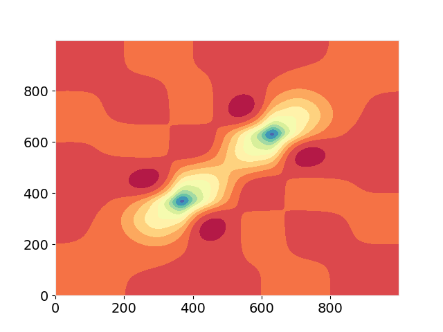
# 2D plot:
fig, ax = plt.subplots(1,1,dpi=100)
ax.contourf(V[0,0,:,0,0,:], levels=11, cmap="Spectral_r")
plt.show()
I obtain the following output and curve:
Total points in mesh 1000
Total points in phi (10, 1000)
Contribution of off-diagonal elements: 52.0181598422788
Integral, diagonal and off-diagonal parts: (-1.018545805226214, -1.4556799511827525)